|
|
|
FAQ
Q1. How is it different from other FOS-based methods such as the mixed formulation?
A. The mixed formulation and FOLSQ are FOS based method, but their systems are not hyperbolic.
Relaxation methods are also FOS based, including the approach proposed in [Gomez et. al. ACME2010],
but their systems are asymptotic approximation to the original PDE, often resulting in stiff relaxation systems.
Yet another is an extension of Cattaneo's hyperbolic heat equations [Montecinos and Toro JCP2014], which
is hyperbolic but again the relaxation time needs to be small, scaled with the mesh size, in order for the hyperbolic system
to model the time-dependent solution accurately.
The first-order hyperbolic system method is different: it is unique in that
the hyperbolic system is constructed such that it recovers the original PDE exactly
in the (pseudo) steady state.
And thus the relaxation time is a free parameter, which is then determined to optimize the convergence to the pseudo steady state, leading to a non-stiff system.
Consequently, numerical schemes generated from the first-order hyperbolic system method cannot be time-accurate with explicit time-stepping schemes; time accurate computations
are possible with implicit time-stepping or space-time schemes. As a matter of distinction, therefore,
if a scheme uses an explicit time-stepping
for unsteady problems, it is not based on the first-order hyperbolic system method.
[ NOTE: Explicit time-integration may be possible. At the time of writing this, no one has tried it. 01-14-2016. ]
Also, the hyperbolic method may be considered as a method for spatial discretization.
It is similar to spatial discretizations of the Euler equations. If you discretize the Euler equations in space
by upwind methods, you assume the Euler equations are hyeprbolic in physical/pseudo time although
they are not hyperbolic in space for subsonic flows. Recall that space-marching methods cannot be applied
to the Euler equations for subsonic flows because they are not fully hyperbolic in space.
Q2. It is computationally expensive, isn't it?
A. It depends on how you measure the cost, on target problems/accuracy, and on what it is compared with.
(1)For 3D Naveir-Stokes, hyperbolic FV schemes require 20 discrete unknowns per cell/node (5 solution variables +
15 gradient variables), which is exactly the same as P1 modal DG. But the hyperbolic scheme achieves one-order higher-order
accuracy in the solution (3rd-order) and the solution gradients (2nd-order) on unstructured grids than the P1 DG, which
is 2nd-order accurate (and 1st-order accurate for the gradients).
See [AIAA2016-1101, AIAA2016-3969 ] for 3D HNS results.
So, the hyperbolic NS scheme should be compared with P2 modal DG (3rd-order with 50 discrete unknwons per cell/node).
(2)For pure diffusion, low-Reynolds-number flows, and highly-resolved boundary layer problems, convergence acceleration
by eliminating second derivatives can yield faster time-to-solution (in CPU time) than conventional 2nd-order schemes on the same grid.
See AIAA2017-0310 for hyperbolic
DG schemes, JCP2014(Diff) for FV schemes,
and AIAA2017-0081 for a boundary layer problem.
In the advection limit, hyperbolic schemes achieve one-order-higher order of accuracy [JCP2014(Adv-Diff)]; and so again
it should be compared with 3rd-order schemes.
(3)For the same discrete problem size (the same number of discrete unknowns), hyperbolic schemes yield more accurate drag preditcion
for viscous problems than a conventional 2nd-order scheme
[AIAA2016-3969 ].
(4) See below for comparisons for 3D Navier-Stokes:
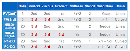
DoFs: Number of discrete unknowns per cell/node for 3D Navier-Stokes (5 variables).
Stiffness: Numerical stiffness due to the viscous terms.
Stencil: Extent of the residual stencil. 1=neighbors only
Quadrature: Flux evaluations. DG methods require volume integrals of fluxes also (Vol).
Remakrs:
- EB(3rd) is applicable only to simplex grids (tetrahedra).
- Exact linearization is possible for all, but JFNK is popular.
- DG is likely to lose compactness if a limiter is applied.
- If 'compact' means that each step is compact, then FV/EB schemes are compact.
- EB(3rd) does not require a high-order mesh, but requires accurate surface normals.
- FV(2nd) requires more than 1 quadrature point for non-triangular faces to keep 2nd-order.
Q3. Is there anything wrong in upwinding the diffusion term?
A. Nothing is wrong. First, upwinding results in a symmetric stencil
due to the symmetric wave structure of the hyperbolic diffusion system, which
is suitable for isotropic diffusion. Second, recall that the hyperbolic diffusion
system is equivalent to the diffusion equation in the steady state or in the absence
of the time derivative. Therefore, the discretization is
consistent with the original diffusion equation in the steady form. You'll be solving the
steady diffusion (or Navier-Stokes) equation correctly. For time-dependent problems,
the hyperbolic discretization is consistent with the time-dependent diffusion equation
at every physical time step, which is a pseudo-steady-state in the implicit formulation
(see CF2014 for
1D problems; AIAA2017-0738 for
3D unsteady Navier-Stokes results).
Q4. What if the numerical scheme does not reach a steady state?
A. It would be a problem. Note that it would be a problem not just for the
hyperbolic method but for many methods, e.g., pseudo-compressible methods, local-preconditioning methods, multigrid methods,
Newton-Krylov methods, any pseudo-time formulation, etc.
For example, you wish to solve a nonlinear equation, N(u)=0, by an iterative method.
What if the iterative method does not converge? Well, it would be a problem.
Q5. What are the disadvantages of the hyperbolic method?
A. It may require more memory than conventional methods because
it expands the governing equations with extra variables. But it actually depends on the discretization method as well as
the solver. For example, it is possible to construct a scheme by reducing
the number of degrees of freedom for some high-order methods (by extending the idea of
Scheme-II ).
Examples can be found in AIAA2017-0310 or in JCP2016 paper [ pdf | journal
].
Another potential disadvantage is the difficulty of the use of explicit time-stepping schemes for time-dependent problems.
If your application does not allow implicit time-stepping or space-time schemes for unsteady computations, then the hyperbolic
method cannot be used because it can be made time accurate only by implicit or space-time schemes.
Q6. Can the hyperbolic method be extended to PDEs involving higher-order derivatives?
A. Yes, but so far, the method has been developed for second-derivatives (diffusion, viscous).
It has been shown that a straightforward extension to third-derivatives leads to
a non-hyperbolic system. However, it is possible to construct a hyperbolic system
by a non-straightforward formulation: See JCP2016 paper for a hyperbolic formulation for
dispersion [ pdf | journal ].
Q7. Is the hyperbolic method applicable to any discretization method, such as DG?
A. Yes, it is. The idea is to reformulate the governing equations. It is independent
of the discretization method. Just remember that the governing equations are made
hyperbolic and thus all you need is a discretization scheme suitable for hyperbolic systems.
See
Development page for some examples: DG methods and Active-flux method.
Q8. How can you construct an upwind scheme for the Navier-Stokes equations
for which the complete eigen-structure has not been found yet?
A. The complete eigen-structure for the hyperbolic NS system is not needed to construct
an upwind scheme. It is possible to construct an upwind scheme
for the hyperbolic viscous terms, and then combine it with an inviscid scheme. The complete eigen-structure for the hyperbolized viscous terms
has been found and described in AIAA2016-1101.
So, an upwind scheme can be constructed for the viscous terms and it can be easily combined with any inviscid scheme.
This approach has been successfully demonstrated for the finite-volume method
in AIAA2011-4043,
JCP2014,
AIAA2014-2091,
AIAA2015-2451 . It is applicable also to the residual-distribution,
and other methods.
Q9. Does the discretization have to be upwind?
A. No, it doesn't have to be. However, a care must be taken to ensure
that the system remains coupled in the discrete level. For example, it is known that
the central-type discretization (no dissipation) decouples the discrete system (i.e., residual) and
all the benefits of the hyperbolic method will be lost as pointed out in Ref.[ JCP2014].
Q10. How should we apply the boundary conditions to the gradient variables?
A.
For 1D diffusion problems, in the case of the Dirichlet problem, one can specify the solution as usual and predict the
gradient by a numerical scheme. In case of the Neumann problem, once can specify the gradient directly
(which is one the variables we carry) just like the Dirichlet condition on the gradient variable, and predict the solution
value by a numerical scheme. This is consistent with the wave structure of the hyperbolic diffusion: always one
characteristic entering into the domain, and so one condition needs to be imposed. It leads to a well-posed
discrete problem as shown in JCP2007.
The same is true in 2D if the gradient is taken as the one normal to the boundary.
The gradient in the tangential direction to the boundary can be either specified (known if the solution is
given along the boundary) or predicted by a numerical scheme.
Below, we show that two boudnary conditons are needed in both the difusion equation and
the hyperbolic formulation [AIAA Paper 2017-0081].
If you consider the one-dimensional diffusion in x=[0,1]:
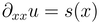
Then, integrate it twice to get

There are two arbitrary constants, c0 and c1, and therefore two boundary consitionds are needed
to determine the solution. The boundary condition is either Dirichlet or Nuemann condition, imposed at
x=0 and x=1. The solution is then uniquely determined.
Now, consider the hyperbolized diffusion:

which becomes in the pseudo steady state:

We integrate it once to get

and therefore, we again need two boundary conditions to determine the solution.
In the same way as in the original problem, the solution is then uniquely determined.
Moreover, it shows that the solution to the first-order system and the solution to the original problem
are identical. Adding additional variable does not change the physical problem and the associated boundary conditions.
See also AIAA2017-0310.
Q11. You are solving a different equation. Is the resulting scheme consistent?
A.
As long as the relaxation time is O(1), on which the hyperbolic method is built,
the resulting discretization is consistent with the target equation in space, i.e.,
in the (pseudo) steady state or when the pseudo time derivative is ignored (e.g., infinite CFL number).
For fully implicit solvers as described in JCP2014,
AIAA2014-2091,
the residual is perfectly consistent with the target equations.
That is, you'll be solving exactly the advection-diffusion and the Navier-Stokes equations.
See also
64th NIA CFD Seminar: "Third-Order Edge-Based Scheme and New Hyperbolic Navier-Stokes System" (pdf) ,
which shows that spatial discretization of hyperbolic Navier-Stokes sytems is consistent with the original Navier-Stokes equations.
(If the relaxation time is taken as
dependent on the mesh spacing, then it is no longer the hyperbolic method considered here, and there is a possibility
that the resulting scheme loses consistency as pointed out in JCP2007.
A carefully defined relaxation time (as a function of mesh spacing) allows the construction of consistent schemes, even
higher-order accuracy as shown by Montecinos and Toro JCP2014. But again that is not the
hyperbolic method considered here. )
Q12. Does the hyperbolized viscous terms generate shock waves?
A.
During the early evolution in the pseudo time, it may, but it should be damped out
quickly towards the pseudo steady state, where the system reduces to the original Navier-Stokes equations.
The original viscous terms are not hyperbolic, and cannot support shock waves.
Q13. The hyperbolic system is equivalent to the diffusion equation in the
steady state. So, the numerical scheme must converge to machine zero to achieve
the equivalence, right?
A. No, it doesn't have to converge to machine zero. Suppose you wish to solve
a nonlinear equation, N(u)=0. Do you need to converge an iterative method to machine zero
to achieve N(u)=0? No, you don't need to because numerical solutions typically converge much faster
than residuals. You can consider also the local-preconditioning method, which manipulates
a time derivative in a PDE to accelerate convergence to a steady state. The manipulated
PDEs is equivalent to the original PDE only in the steady state, but you don't need to converge
numerical schemes to machine zero. Another example would be a Fourier series for a smooth
function represented by an infinite sum of trigonometric functions. Do you really need
infinitely many terms to represent the function accurately? No, you don't need that many because
it usually covnerges quickly, e.g., you wouldn't see any difference after the first 10 terms, depending on the function.
Q14. How do you define the relaxation time Tr?
A.
This is a very important point. Various optimal formulas have been derived:
(1)Optimal formula derived for a residual-distribution scheme to enhance the pseuo-steady cconvergence (require
eigenvalues to be complex conjugate, so that Fourier modes propagate, which is faster than pure damping) [JCP2007] :
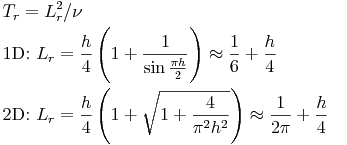
(2)Optimal formula derived by optimizng the condition number of the hyperbolic advection-diffusion system [JCP2010]
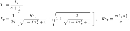
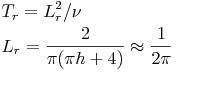
(3)Optimal formula derived by requiring the discrete Fourier mode to propagate in a first-order FV diffusion scheme [JCP2014]
 Currently, the one in (3) is successfully used for the hyperbolic Navier-Stokes system and
the one in Ref.[AIAA Paper 2017-0081] for
high-Reynolds-number boundary layer flows.
Note that the length scale Lr is a nondimensionalized quantity. It should be scaled by the grid length
just like we have to do the same for the Reynolds number. Also, a careful definition is required in the case of solving
dimensional equations. See AIAA Paper 2016-1101 for more details. Also, a specil care is required for high-Reynolds-number boundary-layer flows
(See AIAA Paper 2017-0081).
Currently, the one in (3) is successfully used for the hyperbolic Navier-Stokes system and
the one in Ref.[AIAA Paper 2017-0081] for
high-Reynolds-number boundary layer flows.
Note that the length scale Lr is a nondimensionalized quantity. It should be scaled by the grid length
just like we have to do the same for the Reynolds number. Also, a careful definition is required in the case of solving
dimensional equations. See AIAA Paper 2016-1101 for more details. Also, a specil care is required for high-Reynolds-number boundary-layer flows
(See AIAA Paper 2017-0081).
|
|
|
|
 Hyperbolic Method